Titan terrain from radar
A segmentation network trained to reproduce the six-class global terrain map of Lopes et al. (2020) from the Cassini radar mosaic, then run over the whole mosaic to give a terrain map at 351 m per pixel.
Titan's haze hides the surface from ordinary cameras, so most of what is known about its landscape comes from Cassini's radar. The Lopes map was drawn by hand at global scale. This project asks how much of it a network can recover from the radar alone, and at what level of detail.
The predicted map
The model's terrain classes drawn over the radar mosaic. Black is where Cassini has no radar coverage.
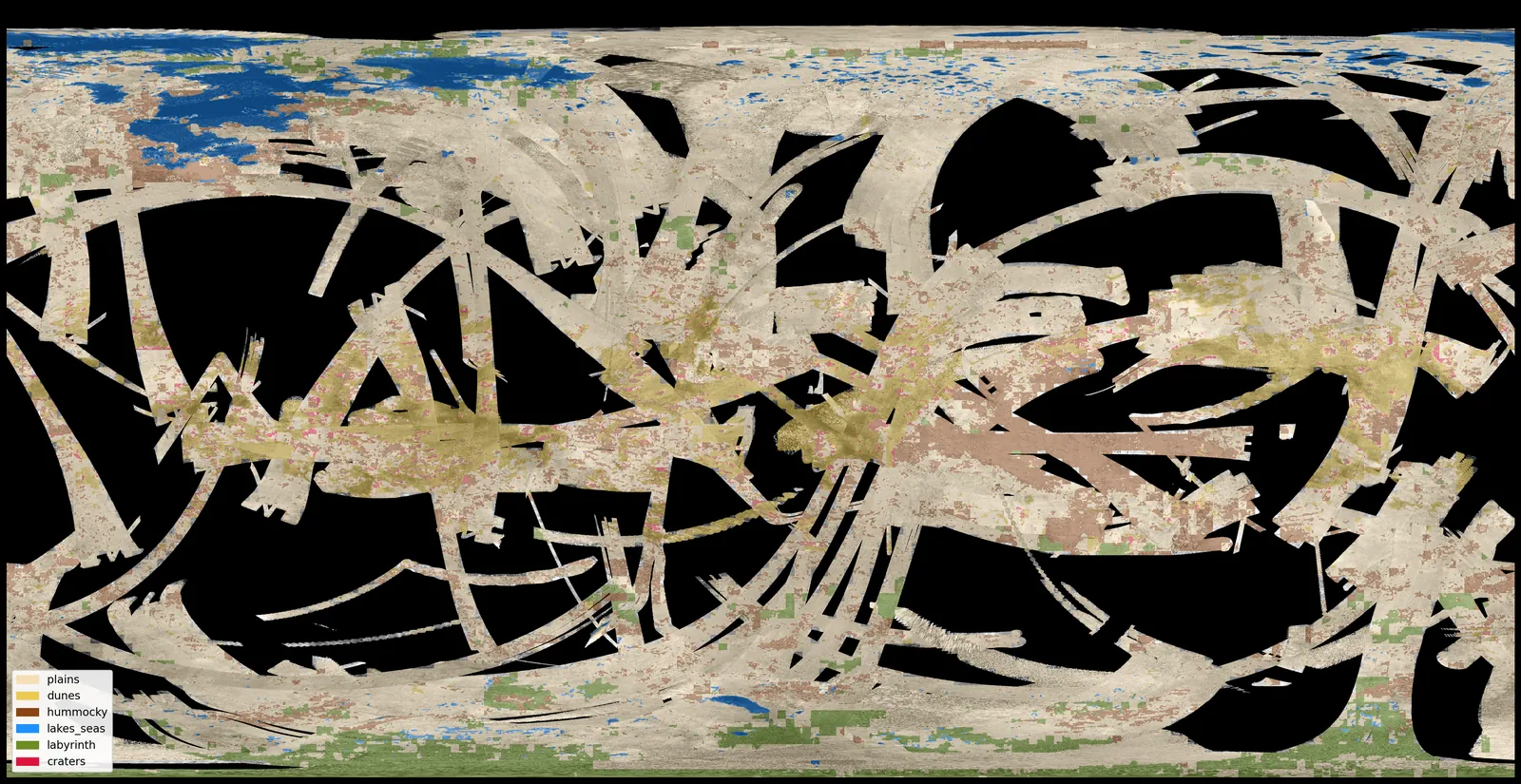
- Plains
- Dunes
- Hummocky / mountainous
- Lakes and seas
- Labyrinth
- Craters
The mosaic is in simple cylindrical projection, so the latitude and longitude readout is approximate. The map is stitched from independent 256-pixel tiles, so seams show when zoomed in.
Results
Mean IoU on a held-out geographic test region, one training run each. Rounds changed different things, so the first two tabs are kept apart on purpose: round 1 and rounds 2 and 3 are not directly comparable. Hover or focus a bar for its caveats.
Round 2 switched to the Lopes 2020 shapefile release and regenerated the train, validation and test split, so the test set changed along with the method. Round 4 (NLDSAR denoised swaths where available) was set up but never evaluated.
Dunes, lakes and plains are learnable from radar texture and brightness. Hummocky and labyrinth terrain are often confused with each other and with plains. Craters cover about 0.3% of the map and are not learned at all.
With one seed per configuration and a test set drawn from a handful of 10 degree blocks, differences of a few hundredths are within run-to-run noise. ImageNet pretraining made almost no difference against random initialisation.
Sample tiles
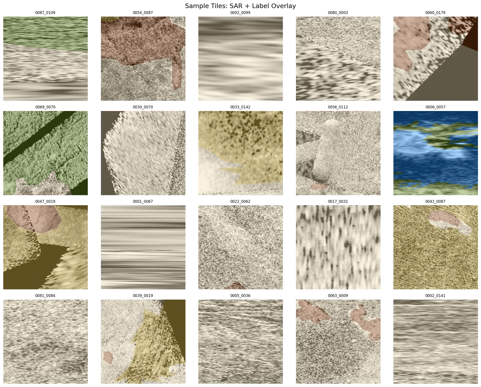
Twenty sample tiles, radar with the label overlaid in the class colours. The streaking in some tiles is the polar distortion described below.
Limitations
- The labels are a map, not ground truth. Lopes et al. drew the map partly from this same radar data, at a scale meant for global interpretation. A high score means agreement with their interpretation, and boundary errors in the map are learned along with it.
- No-radar pixels are scored. Tiles with up to 50% missing radar are kept. Missing pixels are set to zero in the image but keep their map label, so the model is trained and evaluated on some pixels it cannot see. Masking them out is the first fix for the next round, and it will change every number above.
- Polar distortion. The mosaic is in simple cylindrical projection, so tiles near the poles are stretched sideways into streaks. The north polar lakes, which carry most of the lake class, sit in this region.
- Tile edges. The global map is stitched from independent 256-pixel tiles and shows seams.
- 351 m pixels. Fine for regional terrain, far too coarse for anything like landing-site work.
- Round 3 picked its best of several encoders and reported the winner. Its metrics file was not committed; 0.455 is the figure recorded in the round 3 commit.
Related work
Lee (2026), CETUS, uses the same mosaic and Lopes map to benchmark frozen foundation-model encoders on tile-level classification with a longitude-sector split, so its numbers are not comparable to these.